

Introduction
Deep Learning is the subset of Machine Learning and is commonly used to solve complex problems that are otherwise not possible with traditional machine learning methods. And image classification was one such complex task and it was a very challenging task until a few years ago. But with the advancements in Deep Learning and the availability of libraries such as TensorFlow and Pytorch have made deep learning tasks much easier.
In this blog, we’ll use TensorFlow 2 and Keras API to build an end-to-end image classification model using CNN. We assume that you already have theoretical knowledge about Deep Learning and are interested in building an image classification model using TensorFlow 2 and Keras API.
Import libraries
Import all the required modules from Tensorflow and other libraries. The entire code is executed in Kaggle which uses Tensflow version 2.6.2 as of this writting.
					import tensorflow as tf
print(tf.__version__)
					from tensorflow.keras.models import Sequential
from tensorflow.keras.layers import Dense, Flatten, Dropout
from tensorflow.keras.layers import Conv2D, MaxPooling2D
from tensorflow.keras.layers import BatchNormalization
from tensorflow.keras.layers import Rescaling
from tensorflow.keras.layers import RandomFlip, RandomRotation
from tensorflow.keras.regularizers import L2
from tensorflow.keras.preprocessing.image import ImageDataGenerator
					import os
import random
import numpy as np
import pandas as pd
import matplotlib.pyplot as plt
For reproducible results, run the below code at the starting of the code just after all the imports. Note that there will be some operations which have randomness especially when you are using GPU. But, you will get very similar results with the below code.
					SEED = 42
def set_seeds(seed):
    os.environ['PYTHONHASHSEED'] = str(seed)
    random.seed(seed)
    tf.random.set_seed(seed)
    np.random.seed(seed)

def set_global_determinism(seed):
    set_seeds(seed)
    os.environ['TF_DETERMINISTIC_OPS'] = '1'
    os.environ['TF_CUDNN_DETERMINISTIC'] = '1'
    tf.config.threading.set_inter_op_parallelism_threads(1)
    tf.config.threading.set_intra_op_parallelism_threads(1)

set_global_determinism(seed=SEED)
Download dataset
We’ll be using Cat and Dog dataset for this tutorial and is available on Kaggle. The dataset contains two folders – training_set and test_set. The dataset structure is shown below –
					└── cat-and-dog
        ├── test_set
        │   └── test_set
        │       ├── cats
        │       ├── dogs
        ├── training_set
        │   └── training_set
        │       ├── cats
        │       ├── dogs
The training_set contains 4001 cat images and 4006 dog images.
					train_cats = len(os.listdir("../input/cat-and-dog/training_set/training_set/cats"))
train_dogs = len(os.listdir("../input/cat-and-dog/training_set/training_set/dogs"))
print(f'The training dataset contains {train_cats} cat images and {train_dogs} dog images')
The training dataset contains 4001 cat images and 4006 dog images
The test_set contains 1012 cat images and 1013 dog images. We won’t be using test_set data for training as the same suggests it will only be used for prediction and validating the results.
					test_cats = len(os.listdir("../input/cat-and-dog/test_set/test_set/cats"))
test_dogs = len(os.listdir("../input/cat-and-dog/test_set/test_set/dogs"))
print(f'The test dataset contains {test_cats} cat images and {test_dogs} dog images')
The test dataset contains 1012 cat images and 1013 dog images
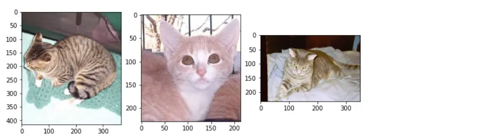
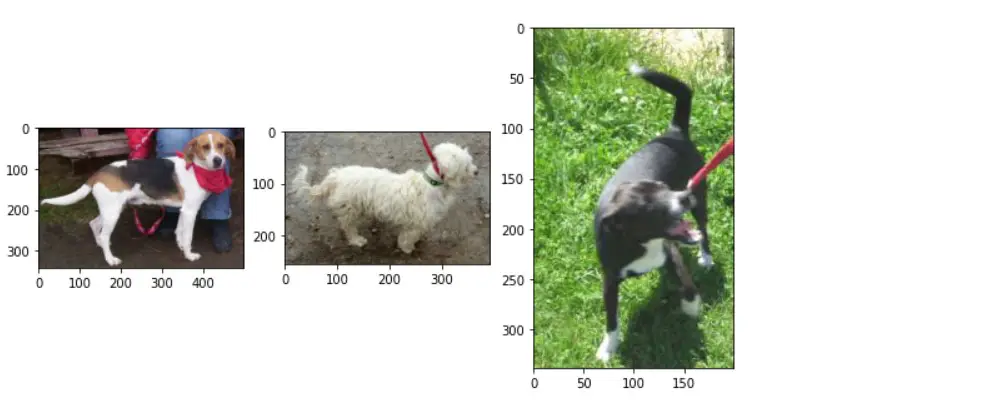
We have seen the directory structure. Let’s look at few images from both the classes – Cats and Dogs. From the below code, we randomly selected 3 images from both categories. Notice that the dataset contains images with different dimensions. But Neural Networks expect images of fixed dimensions. You’ll see how to deal with challenge shortly.
					fig, axes = plt.subplots(nrows=1, ncols=3, figsize=(10, 5))
path = "../input/cat-and-dog/training_set/training_set/cats"

for i, ax in enumerate(axes.flat):
    files = random.choices(os.listdir(path), k=3)
    files = [path+'/'+file for file in files]
    ax.imshow(plt.imread(files[i]))
					fig, axes = plt.subplots(nrows=1, ncols=3, figsize=(10, 5))

path = "../input/cat-and-dog/training_set/training_set/dogs"
for i, ax in enumerate(axes.flat):
    files = random.choices(os.listdir(path), k=3)
    files = [path+'/'+file for file in files]
    ax.imshow(plt.imread(files[i]))
Create a dataset
So far, we have imported all the libraries and explored the dataset. Next, we need to create dataset object to read the images from directories. But, we have one small problem to tackle. As you have seen above, the dataset contains images of varying sizes. But the input to CNN requires images with fixed dimension, say 64×64 or 128×128 or 299×299, etc. To convert all the images to same size we’re setting the image_size parameter to 299×299 so that when reading images from the directory they will be converted to a fixed dimension of our choice on the fly.
					IMG_HEIGHT = 299
IMG_WIDTH = 299
BATCH_SIZE = 32
To create dataset generator objects that read images from the directory. we’ll be using tf.keras.utils.image_dataset_from_directory. The image_dataset_from_directory supports many keyword parameters as you can see in the below example. The parameters are self-explanatory. For additional details on image_dataset_from_director, refer here.
Note that we are splitting train data into training and validation set with 85:15 ratio.
					train_ds = tf.keras.utils.image_dataset_from_directory(
    directory="../input/cat-and-dog/training_set/training_set",
    label_mode='categorical',
    color_mode='rgb',
    batch_size=BATCH_SIZE,
    image_size=(IMG_HEIGHT, IMG_WIDTH),
    shuffle=True,
    seed=SEED,
    validation_split=0.15,
    subset='training'
)
					Found 8005 files belonging to 2 classes.
Using 6805 files for training.
					valid_ds = tf.keras.utils.image_dataset_from_directory(
    directory="../input/cat-and-dog/training_set/training_set",
    label_mode='categorical',
    color_mode='rgb',
    batch_size=BATCH_SIZE,
    image_size=(IMG_HEIGHT, IMG_WIDTH),
    shuffle=True,
    seed=SEED,
    validation_split=0.15,
    subset='validation'
)
					Found 8005 files belonging to 2 classes.
Using 1200 files for validation.
					test_ds = tf.keras.utils.image_dataset_from_directory(
    directory="../input/cat-and-dog/test_set/test_set",
    label_mode='categorical',
    color_mode='rgb',
    batch_size=BATCH_SIZE,
    image_size=(IMG_HEIGHT, IMG_WIDTH),
    shuffle=True,
    seed=SEED,
)
Found 2023 files belonging to 2 classes.
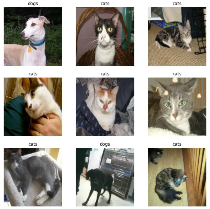
Let’s look at the few images again. This time we will use train_ds so that we can see resized images because we used fixed image_size of 299×299. As you can see from the below, all the images are resized.
					import matplotlib.pyplot as plt

plt.figure(figsize=(10, 10))
for images, labels in train_ds.take(1):
    for i in range(9):
        ax = plt.subplot(3, 3, i + 1)
        plt.imshow(images[i].numpy().astype("uint8"))
        plt.title(class_names[labels[i].numpy()[1].astype("uint8")])
        plt.axis("off")
Basic model
Its now time to create the model. We are going to create a very simple CNN and then try to improve the model in the next section i.e. Dealing with overfitting.
Create a model
The below CNN model consists of 2 Convolution layers followed by MaxPooling layers, then Flatten and finally 2 Dense layer. The final Dense layer outputs probability for cat and dog classes.
					num_classes = len(class_names)

model = Sequential([
    Rescaling(1./255, input_shape=(IMG_HEIGHT, IMG_WIDTH, 3)),
    Conv2D(64, (3,3), activation='relu'),
    MaxPooling2D((3,3)),
    Conv2D(32, (3,3), activation='relu'),
    MaxPooling2D((3,3)),
    Flatten(),
    Dense(128, activation='relu'),
    Dense(num_classes, activation='softmax')
])
Next run model.summary() method which gives summary of the model –
model.summary()
					Model: "sequential"
_________________________________________________________________
Layer (type)                 Output Shape              Param #
=================================================================
rescaling (Rescaling)        (None, 299, 299, 3)       0
_________________________________________________________________
conv2d (Conv2D)              (None, 297, 297, 64)      1792
_________________________________________________________________
max_pooling2d (MaxPooling2D) (None, 99, 99, 64)        0
_________________________________________________________________
conv2d_1 (Conv2D)            (None, 97, 97, 32)        18464
_________________________________________________________________
max_pooling2d_1 (MaxPooling2 (None, 32, 32, 32)        0
_________________________________________________________________
flatten (Flatten)            (None, 32768)             0
_________________________________________________________________
dense (Dense)                (None, 128)               4194432
_________________________________________________________________
dense_1 (Dense)              (None, 2)                 258
=================================================================
Total params: 4,214,946
Trainable params: 4,214,946
Non-trainable params: 0
_________________________________________________________________
Compile the model
Next, we need to compile the model by passing optimizer, loss and evaluation metric. You can either directly pass the values as string (method 1) or by explicitly using tf.keras (tf.keras.optimizers. or tf.keras.losses. or tf.keras.metrics.). You can also pass multiple evaluation metrics to metrics parameter but to keep it simple we are only passing categorical_accuracy metric.
					# Method 1
# model.compile(
#     optimizer='adam',
#     loss='categorical_crossentropy',
#     metrics=['categorical_accuracy']
# )

# Method 2
model.compile(
    optimizer=tf.keras.optimizers.Adam(learning_rate=0.001),
    loss=tf.keras.losses.CategoricalCrossentropy(),
    metrics=[tf.keras.metrics.categorical_accuracy]
)
Train the model
This below code tells how train_ds (and valid_ds) are used during training the model. As you can see from the output –
- 32 – batch size. This means that each time 32 images are read from the directory and fed to network
- 299, 299 – image dimension
- 3 – channels
					for image_batch, labels_batch in train_ds:
     print(image_batch.shape)
     print(labels_batch.shape)
     break
					(32, 299, 299, 3)
(32, 2)
Next, train the model for 10 epochs. Note that we are assigning model.fit() to history. As the model is running, the logs are stored in history and used to visualize the loss and metrics which you see in next.
					history = model.fit(
    train_ds,
    validation_data=valid_ds,
    batch_size=BATCH_SIZE,
    epochs=10
)
					Epoch 1/10
2022-11-08 14:15:23.710464: I tensorflow/stream_executor/cuda/cuda_dnn.cc:369] Loaded cuDNN version 8005
213/213 [==============================] - 41s 153ms/step - loss: 0.7355 - categorical_accuracy: 0.5616 - val_loss: 0.6648 - val_categorical_accuracy: 0.6200
Epoch 2/10
213/213 [==============================] - 25s 116ms/step - loss: 0.6459 - categorical_accuracy: 0.6331 - val_loss: 0.6530 - val_categorical_accuracy: 0.6450
Epoch 3/10
213/213 [==============================] - 20s 94ms/step - loss: 0.5684 - categorical_accuracy: 0.7021 - val_loss: 0.6395 - val_categorical_accuracy: 0.6658
Epoch 4/10
213/213 [==============================] - 21s 95ms/step - loss: 0.4619 - categorical_accuracy: 0.7735 - val_loss: 0.6902 - val_categorical_accuracy: 0.6725
Epoch 5/10
213/213 [==============================] - 21s 96ms/step - loss: 0.3389 - categorical_accuracy: 0.8572 - val_loss: 0.8541 - val_categorical_accuracy: 0.6567
Epoch 6/10
213/213 [==============================] - 20s 94ms/step - loss: 0.1909 - categorical_accuracy: 0.9270 - val_loss: 1.1586 - val_categorical_accuracy: 0.6425
Epoch 7/10
213/213 [==============================] - 21s 97ms/step - loss: 0.1217 - categorical_accuracy: 0.9577 - val_loss: 1.4077 - val_categorical_accuracy: 0.6358
Epoch 8/10
213/213 [==============================] - 21s 96ms/step - loss: 0.0678 - categorical_accuracy: 0.9799 - val_loss: 1.5085 - val_categorical_accuracy: 0.6408
Epoch 9/10
213/213 [==============================] - 21s 95ms/step - loss: 0.0445 - categorical_accuracy: 0.9890 - val_loss: 1.6920 - val_categorical_accuracy: 0.6383
Epoch 10/10
213/213 [==============================] - 25s 116ms/step - loss: 0.0357 - categorical_accuracy: 0.9902 - val_loss: 2.2332 - val_categorical_accuracy: 0.6475
Training logs are imported into dataframe df and used to visualize the training and validation loss & accuracy.
df = pd.DataFrame(history.history)
					acc = history.history['categorical_accuracy']
val_acc = history.history['val_categorical_accuracy']

loss = history.history['loss']
val_loss = history.history['val_loss']

epochs_range = range(10)

plt.figure(figsize=(15, 7))
plt.subplot(1, 2, 1)
plt.plot(epochs_range, loss, label='Training Loss')
plt.plot(epochs_range, val_loss, label='Validation Loss')
plt.legend(loc='upper right')
plt.title('Training and Validation Loss')

plt.subplot(1, 2, 2)
plt.plot(epochs_range, acc, label='Training Accuracy')
plt.plot(epochs_range, val_acc, label='Validation Accuracy')
plt.legend(loc='lower right')
plt.title('Training and Validation Accuracy')
plt.figure(figsize=(10, 6));
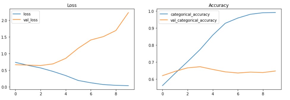
The above visualization shows that training and validation accuracy are not in sync. The training accuracy is about 99% but validation accuracy is just about 65% which is a clear indication of model overfitting.
So, in the next section, we will look into how to deal with overfitting.
Evaluate the model
The above basic CNN model gives only 65% on unseen data i.e. test data. Though it is close to validation accuracy the model has overfit the training data and failed to generalize well on the test data. Let’s see how we can improve the model further in the next section.
model.evaluate(test_ds, batch_size=32, verbose=1)
					64/64 [==============================] - 9s 115ms/step - loss: 2.1651 - categorical_accuracy: 0.6535

[2.165060520172119, 0.6534849405288696]
Dealing with overfitting
One of the challenges with deep learning models is overfitting. Overfitting happens when the model fails to generalize on the new unseen data. As seen from the previous section, our model has overfit the data and there is a huge difference in accuracy between training and validation data. In this section, let’s improve the model performance using the options available in TensorFlow and Keras API.
Here are some of the methods to deal with overfitting. In this post, we will use augmented data, adding dropout layer & regularizers, and improving the model architecture –
- Increase the dataset size
- Augmented data
- Adding dropout layers
- Adding regularization
- Improve the model architecture
- Pre-trained models, etc.
Data augmentation
Data augmentation is the technique to create additional images by applying random transformations such as random crop, random zoom, random flip, etc. In this example, RandomFlip and RandomRotation methods are applied. There are many other functions available under tf.keras.layers.
					data_augmentation = Sequential([
    RandomFlip("horizontal", input_shape=(IMG_HEIGHT, IMG_WIDTH, 3)),
    RandomRotation(0.1)
])
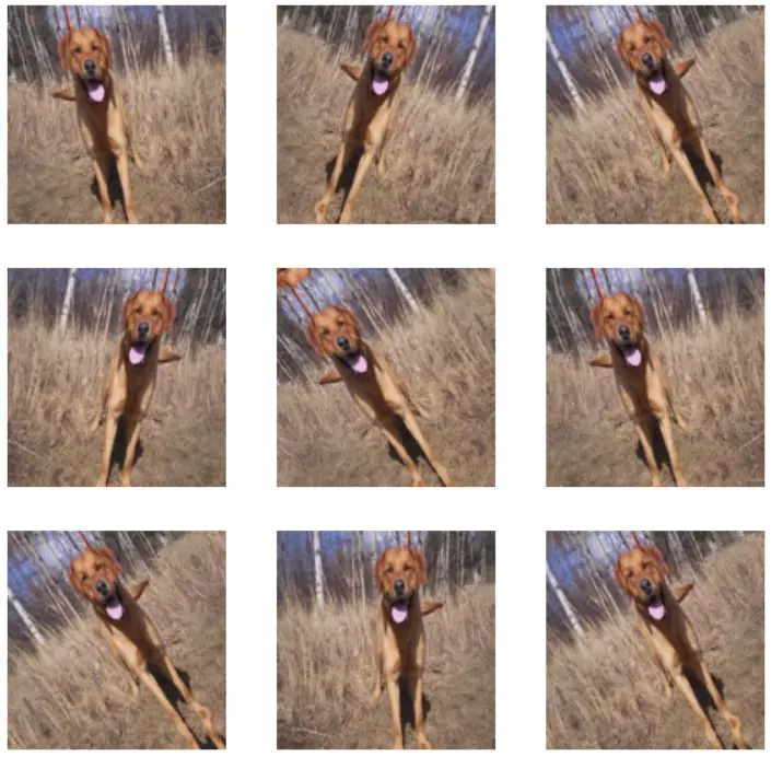
The below visualization shows data augmentation applied to one of the images 9 times.
					plt.figure(figsize=(10, 10))
for images, _ in train_ds.take(1):
    for i in range(9):
        augmented_images = data_augmentation(images)
        ax = plt.subplot(3, 3, i + 1)
        plt.imshow(augmented_images[0].numpy().astype("uint8"))
        plt.axis("off")
Regularization, Dropout and updated Model
The below changes done to the base model to deal with overfitting and improve the model performance.
- Data augmentation layer is added as the first layer in the model
- L2 regularization is added to Conv2D and Dense layers
- 3 Dropout layers are added
					num_classes = len(class_names)

model = Sequential([
    data_augmentation,
    Rescaling(1./255),
    Conv2D(64, (3,3), activation='relu', kernel_regularizer=L2(1e-5)),
    MaxPooling2D((3,3)),
    Dropout(0.2),
    Conv2D(32, (3,3), activation='relu', kernel_regularizer=L2(1e-5)),
    MaxPooling2D((3,3)),
    Dropout(0.2),
    Conv2D(32, (3,3), activation='relu', kernel_regularizer=L2(1e-5)),
    MaxPooling2D((3,3)),
    Dropout(0.2),
    Flatten(),
    Dense(64, activation='relu', kernel_regularizer=L2(1e-5)),
    Dense(num_classes, activation='softmax')
])
Compile the new model –
					model.compile(
    optimizer=tf.keras.optimizers.Adam(learning_rate=0.001),
    loss=tf.keras.losses.CategoricalCrossentropy(),
    metrics=[tf.keras.metrics.categorical_accuracy]
)
And then train the model for 15 epochs –
					EPOCHS = 15
history = model.fit(
    train_ds,
    validation_data=valid_ds,
    batch_size=32,
    epochs=EPOCHS
)
					Epoch 1/15
213/213 [==============================] - 28s 124ms/step - loss: 0.6880 - categorical_accuracy: 0.5628 - val_loss: 0.6698 - val_categorical_accuracy: 0.6375
Epoch 2/15
213/213 [==============================] - 26s 122ms/step - loss: 0.6623 - categorical_accuracy: 0.6126 - val_loss: 0.6066 - val_categorical_accuracy: 0.6925
Epoch 3/15
213/213 [==============================] - 21s 96ms/step - loss: 0.6296 - categorical_accuracy: 0.6417 - val_loss: 0.5876 - val_categorical_accuracy: 0.6883
Epoch 4/15
213/213 [==============================] - 21s 97ms/step - loss: 0.6034 - categorical_accuracy: 0.6732 - val_loss: 0.5728 - val_categorical_accuracy: 0.6992
Epoch 5/15
213/213 [==============================] - 21s 96ms/step - loss: 0.5733 - categorical_accuracy: 0.6960 - val_loss: 0.5264 - val_categorical_accuracy: 0.7350
Epoch 6/15
213/213 [==============================] - 21s 97ms/step - loss: 0.5511 - categorical_accuracy: 0.7217 - val_loss: 0.4863 - val_categorical_accuracy: 0.7775
Epoch 7/15
213/213 [==============================] - 21s 96ms/step - loss: 0.5208 - categorical_accuracy: 0.7424 - val_loss: 0.5147 - val_categorical_accuracy: 0.7308
Epoch 8/15
213/213 [==============================] - 21s 98ms/step - loss: 0.5089 - categorical_accuracy: 0.7474 - val_loss: 0.4807 - val_categorical_accuracy: 0.7700
Epoch 9/15
213/213 [==============================] - 22s 98ms/step - loss: 0.4899 - categorical_accuracy: 0.7625 - val_loss: 0.4461 - val_categorical_accuracy: 0.8058
Epoch 10/15
213/213 [==============================] - 26s 119ms/step - loss: 0.4659 - categorical_accuracy: 0.7735 - val_loss: 0.4522 - val_categorical_accuracy: 0.7758
Epoch 11/15
213/213 [==============================] - 21s 96ms/step - loss: 0.4490 - categorical_accuracy: 0.7872 - val_loss: 0.4323 - val_categorical_accuracy: 0.7983
Epoch 12/15
213/213 [==============================] - 21s 96ms/step - loss: 0.4431 - categorical_accuracy: 0.7900 - val_loss: 0.4421 - val_categorical_accuracy: 0.7958
Epoch 13/15
213/213 [==============================] - 21s 97ms/step - loss: 0.4387 - categorical_accuracy: 0.7940 - val_loss: 0.4285 - val_categorical_accuracy: 0.8100
Epoch 14/15
213/213 [==============================] - 22s 99ms/step - loss: 0.4202 - categorical_accuracy: 0.8054 - val_loss: 0.4188 - val_categorical_accuracy: 0.8250
Epoch 15/15
213/213 [==============================] - 21s 94ms/step - loss: 0.4140 - categorical_accuracy: 0.8072 - val_loss: 0.4543 - val_categorical_accuracy: 0.7983
df = pd.DataFrame(history.history)
					acc = history.history['categorical_accuracy']
val_acc = history.history['val_categorical_accuracy']

loss = history.history['loss']
val_loss = history.history['val_loss']

epochs_range = range(15)

plt.figure(figsize=(15, 7))
plt.subplot(1, 2, 1)
plt.plot(epochs_range, loss, label='Training Loss')
plt.plot(epochs_range, val_loss, label='Validation Loss')
plt.legend(loc='upper right')
plt.title('Training and Validation Loss')

plt.subplot(1, 2, 2)
plt.plot(epochs_range, acc, label='Training Accuracy')
plt.plot(epochs_range, val_acc, label='Validation Accuracy')
plt.legend(loc='lower right')
plt.title('Training and Validation Accuracy')
plt.figure(figsize=(10, 6));
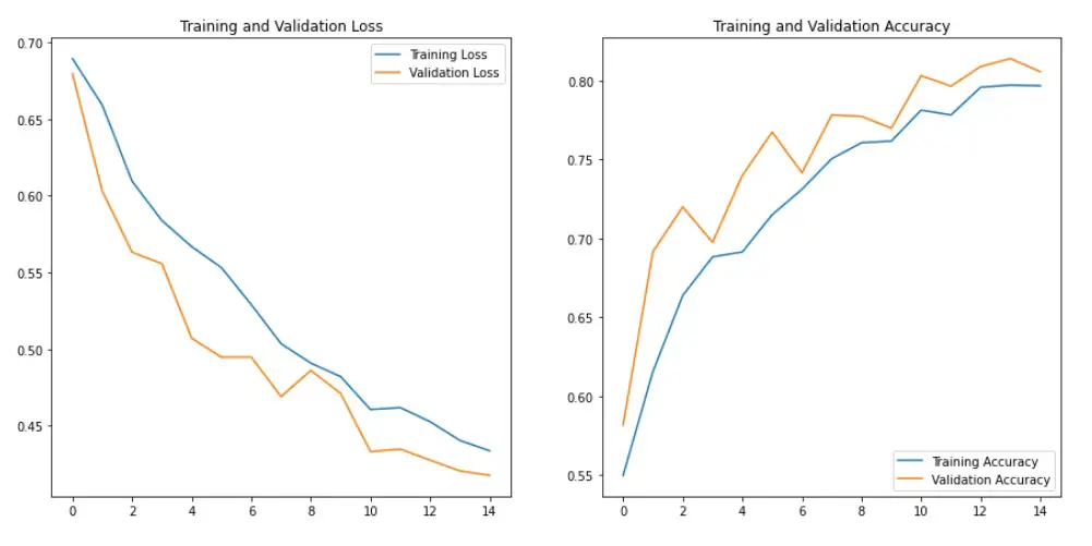
As seen from the above visualization, the difference between training and validation accuracy has reduced and now are in sync. This indicates that we have dealt with overfitting.
Evaluate the model on unseen (test) data –
model.evaluate(test_ds, batch_size=32, verbose=1)
					64/64 [==============================] - 5s 71ms/step - loss: 0.4454 - categorical_accuracy: 0.8028
[0.4453931450843811, 0.8027681708335876]
Overall, the model accuracy on validation set and unseen data (test data) has improved significatly from ~65% to ~80% accuracy.
Prediction
We now have good image classifier built using TensorFlow 2 and Keras API that can predict cat or dog images with 80% accuracy. With model.predict() method we can predict on the entire test data and store the results in predictions.
					predictions = model.predict(test_ds)
predictions = np.round(predictions)
print(predictions)
					array([[1., 0.],
       [0., 1.],
       [0., 1.],
       ...,
       [0., 1.],
       [1., 0.],
       [1., 0.]], dtype=float32)
If you want to predict on a single image that is not part of the validation or test set, then you can use the below code –
					img_url = "https://upload.wikimedia.org/wikipedia/commons/1/12/Tabby_cat_with_visible_nictitating_membrane.jpg"
img_path = tf.keras.utils.get_file(origin=img_url)

img = tf.keras.utils.load_img(img_path, target_size=(IMG_HEIGHT, IMG_WIDTH))
img_array = tf.keras.utils.img_to_array(img)
img_array = tf.expand_dims(img_array, 0)

predictions = model.predict(img_array)
score = tf.nn.softmax(predictions[0])

print(
    "This image most likely belongs to {} with a {:.2f} percent confidence."
    .format(class_names[np.argmax(score)], 100 * np.max(score))
)
This image most likely belongs to cats with a 72.86 percent confidence.
Save model
The final model can be saved using model.save() method. You can save the entire model in 2 different ways. But TensorFlow SavedModel method is recommended for saving the model.
- Keras .h5 format or
- TensorFlow SavedModel format.
					model.save('tf_model.h5')

!ls
tf_model.h5
The Tensorflow SavedModel method the default method. So if you don’t pass any extension, TensorFlow will create below files and folders. when saving the model. The model architecture and training configuration (including the optimizer, losses, and metrics) are stored in saved_model.pb. The weights are saved in the variables directory.
					model.save('my_model')

!ls my_model
assets keras_metadata.pb saved_model.pb variables
Load model
Both Keras .h5 model and TensorFlow SavedModel models can be loaded using load_model() method as shown below.
					from tensorflow.keras.models import load_model

# Load Keras model
model = load_model('tf_model.h5')

# Load TensorFlow SavedModel
model = load_model('my_model')
Summary
We can still try to improve the model by trying out different data augmentation techniques, building a deep neural network, training for more epochs, fine-tuning, adding dropout and different regularizers, etc. In the next kernel, let’s see if we can improve the model using transfer learning.
