

Introduction
Transfer learning is a widely used technique in Deep Learning to solve complex computer vision and NLP tasks. Building a powerful and complex deep-learning model needs a lot of data. Even if we have access to data it requires a lot of computing power and time. More importantly the cost associated. This is where transfer learning shines. Let’s see how we use transfer learning for image classification in this article.
In the previous article, we built an image classification model to classify cats and dogs using TensorFlow 2 and Keras API with 80% accuracy without transfer learning. The goal of this blog is how we can further improve the accuracy by making use of transfer learning. You’ll be amazed to see the result of transfer learning. This blog can be considered as Part 2 of Image Classification using CNN and TensorFlow 2.
What is transfer learning?
Transfer learning is a technique in which the model trained on one task is re-used for another task. The most popular example of transfer learning in computer vision is models trained on imagenet dataset. These models are trained on more than 14 million images covering 1000 categories. Training these models takes a lot of computing power, time, and cost. With the help of transfer learning you can re-use the learning from already trained model with almost no cost to you.
There are 2 ways we can use pre-trained models for transfer learning as described below –
(a) Method 1 – Feature Extraction: In this method, the pre-trained model is used without final classifier layers (layers from Flatten) because the pre-trained model is trained on one task (for example, imagenet data which has 1000 classes) and we are using it for another task which may not have 1000 classes to predict. So, we have to add the final classifier layers on top of the pre-trained model as per our requirements.
The below image shows all the layers for VGG16 architecture. In this method, we only remove the final classifier layers (4 layers) and add the classifier layer as per the requirement.
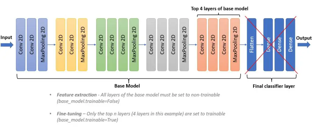
(b) Method 2 – Fine-tuning: Fine-tuning is very similar to the feature extraction method. But, along with adding the classifier layer, a few of the top layers of the base model are set to trainable. So when we train the model, the final classifier layer along with the last few layers of the base model is also gets trained.
In the above diagram of VGG16 architecture, the base model is referred to all the layers except the final classifier. Here the top 4 layers of the base model are set to trainable. So when we train this model after adding the final classifier, only the top 4 layers and final classifier layers will be trained and weights get updated accordingly.
Now, let’s just jump to the practical implementation of transfer learning using VGG16 with TensorFlow2.
Transfer Learning for Image Classification
There are about 40+ pre-trained models that are trained on imagenet data and the details about these models can be found here. Some of the pre-trained models are — VGG16, VGG19, ResNet, DenseNet, EfficientNet, etc. You should explore as many as possible to see how it performs on your data. For this blog, we will be using the VGG16.
Transfer learning with VGG16 (feature extraction method)
The code is almost similar if you have already gone through our previous blog here. We’ll concentrate mainly on how transfer learning is done in this article.
Import libraries
					import os
import random
import numpy as np
import pandas as pd
import matplotlib.pyplot as plt
import tensorflow as tf
from tensorflow.keras.models import Sequential
from tensorflow.keras.layers import Dense, Flatten, Dropout
from tensorflow.keras.layers import Conv2D, MaxPooling2D
from tensorflow.keras.layers import BatchNormalization
from tensorflow.keras.layers import Rescaling
from tensorflow.keras.layers import RandomFlip, RandomRotation, RandomZoom
from tensorflow.keras.regularizers import L2
Download and create the dataset
As per the documentation, VGG16 supports any input size greater than 32 x 32. Our dataset has images of varying dimensions but we’ll stick with an image dimension of 224 x 224.
					IMG_HEIGHT = 224
IMG_WIDTH = 224
BATCH_SIZE = 32
Next, create train_ds, valid_ds, and test_ds generator objects using image_dataset_from_directory. Note that we are using 85% of the data for training and the remaining 15% for validation. The test_ds is considered unseen data on which we validate the model’s accuracy.
					train_ds = tf.keras.utils.image_dataset_from_directory(
    directory="../input/cat-and-dog/training_set/training_set",
    label_mode='categorical',
    color_mode='rgb',
    batch_size=BATCH_SIZE,
    image_size=(IMG_HEIGHT, IMG_WIDTH),
    shuffle=True,
    seed=SEED,
    validation_split=0.15,
    subset='training'
)

valid_ds = tf.keras.utils.image_dataset_from_directory(
    directory="../input/cat-and-dog/training_set/training_set",
    label_mode='categorical',
    color_mode='rgb',
    batch_size=BATCH_SIZE,
    image_size=(IMG_HEIGHT, IMG_WIDTH),
    shuffle=True,
    seed=SEED,
    validation_split=0.15,
    subset='validation'
)
					Found 8005 files belonging to 2 classes.
Using 6805 files for training.

Found 8005 files belonging to 2 classes.
Using 1200 files for validation.
					test_ds = tf.keras.utils.image_dataset_from_directory(
    directory="../input/cat-and-dog/test_set/test_set",
    label_mode='categorical',
    color_mode='rgb',
    batch_size=BATCH_SIZE,
    image_size=(IMG_HEIGHT, IMG_WIDTH),
    shuffle=True,
    seed=SEED,
)
Found 2023 files belonging to 2 classes
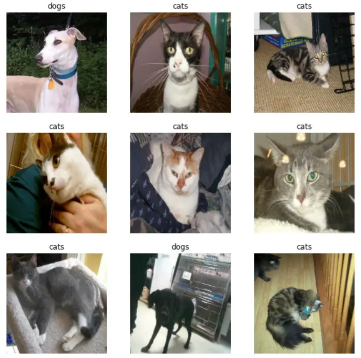
The below code shows sample images from train_ds. Notice that all images have been resized to a common dimension of 244×244.
					import matplotlib.pyplot as plt

plt.figure(figsize=(10, 10))
for images, labels in train_ds.take(1):
    for i in range(9):
        ax = plt.subplot(3, 3, i + 1)
        plt.imshow(images[i].numpy().astype("uint8"))
       plt.title(class_names[labels[i].numpy()[1].astype("uint8")])
        plt.axis("off")
Create the model
The below code will download the VGG16 pre-trained model. As you download the model, weights are initialized with imagenet trained weights and the final classifier layers are not included in the model. Refer below –
					IMG_SHAPE = (IMG_HEIGHT, IMG_WIDTH) + (3,)

base_model = tf.keras.applications.mobilenet_v2(input_shape=IMG_SHAPE,
                                                include_top=False,
                                                weights='imagenet')
					Downloading data from https://storage.googleapis.com/tensorflow/keras-applications/vgg16/vgg16_weights_tf_dim_ordering_tf_kernels_notop.h5
58892288/58889256 [==============================] - 0s 0us/step
58900480/58889256 [==============================] - 0s 0us/step
- input_shape — input shape of the image in the format (height, width, channels).
- include_top — if set to True all the layers are included otherwise final classifier layers are not included.
- weights — If set to ‘imagenet’, pre-trained weights are loaded otherwise weights are initialized randomly.
Next, we need to set base_model.trainable attribute of the model to False . This is a very important step. This means that all the layers of the downloaded pre-trained model are frozen and they won’t get updated during the training. If you don’t set this False then during the training all the weights learned during imagenet training will be lost and you’ll be basically training VGG16 layers from scratch without any transfer learning.
Next, using TensorFlow’s functional API, the GlobalAveragePooling layer, the Dropout layer, and finally, a Dense layer with 2 outputs is added on top of the base model. These layers we call as final classifier layers. And before the base model, we added data_augmentation and processing steps.
					base_model.trainable = False
preprocess_input = tf.keras.applications.vgg16.preprocess_input

inputs = tf.keras.Input(shape=(IMG_HEIGHT, IMG_WIDTH, 3))
x = data_augmentation(inputs)
x = preprocess_input(x)
x = base_model(x, training=False)
x = tf.keras.layers.GlobalAveragePooling2D()(x)
x = tf.keras.layers.Dropout(0.1)(x)
outputs = tf.keras.layers.Dense(2, activation='softmax')(x)
model = tf.keras.Model(inputs, outputs)
Compile
Compile the model using Adam optimizer, Categorical Crossentropy loss, and categorial accuracy.
					model.compile(
    optimizer=tf.keras.optimizers.Adam(learning_rate=0.001),
    loss=tf.keras.losses.CategoricalCrossentropy(),
    metrics=[tf.keras.metrics.categorical_accuracy]
)
Train
Next, train the model for 5 epochs. Notice that in the epoch itself we are able to achieve about 98% accuracy on both training and validation.
					EPOCHS = 5
history = model.fit(
    train_ds,
    validation_data=valid_ds,
    batch_size=32,
    epochs=EPOCHS
)
					Epoch 1/5
2022-11-15 05:19:42.231343: I tensorflow/stream_executor/cuda/cuda_dnn.cc:369] Loaded cuDNN version 8005
213/213 [==============================] - 41s 154ms/step - loss: 0.6098 - categorical_accuracy: 0.8796 - val_loss: 0.0753 - val_categorical_accuracy: 0.9733
Epoch 2/5
213/213 [==============================] - 23s 105ms/step - loss: 0.2292 - categorical_accuracy: 0.9465 - val_loss: 0.0577 - val_categorical_accuracy: 0.9800
Epoch 3/5
213/213 [==============================] - 24s 112ms/step - loss: 0.1656 - categorical_accuracy: 0.9581 - val_loss: 0.0326 - val_categorical_accuracy: 0.9875
Epoch 4/5
213/213 [==============================] - 23s 106ms/step - loss: 0.1537 - categorical_accuracy: 0.9602 - val_loss: 0.0387 - val_categorical_accuracy: 0.9850
Epoch 5/5
213/213 [==============================] - 23s 105ms/step - loss: 0.1305 - categorical_accuracy: 0.9644 - val_loss: 0.0305 - val_categorical_accuracy: 0.9867
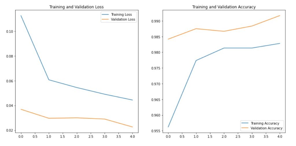
Let’s plot the loss and accuracy to check if we are overfitting the data. As you can see, the accuracy for training and validation are close to each other confirming that there is no sign of overfitting.
					df = pd.DataFrame(history.history)

acc = history.history['categorical_accuracy']
val_acc = history.history['val_categorical_accuracy']
loss = history.history['loss']
val_loss = history.history['val_loss']
epochs_range = range(5)

plt.figure(figsize=(15, 7))

plt.subplot(1, 2, 1)
plt.plot(epochs_range, loss, label='Training Loss')
plt.plot(epochs_range, val_loss, label='Validation Loss')
plt.legend(loc='upper right')
plt.title('Training and Validation Loss')

plt.subplot(1, 2, 2)
plt.plot(epochs_range, acc, label='Training Accuracy')
plt.plot(epochs_range, val_acc, label='Validation Accuracy')
plt.legend(loc='lower right')
plt.title('Training and Validation Accuracy')
plt.figure(figsize=(10, 6));
Evaluate
The accuracy of the unseen data (test data) is around 98%. Our classification model is working as expected.
model.evaluate(test_ds, batch_size=32, verbose=1)
					64/64 [==============================] - 9s 119ms/step - loss: 0.0798 - categorical_accuracy: 0.9827
[0.07984083145856857, 0.9826989769935608]
Prediction
To get predictions for all the test samples use the below code.
					predictions = model.predict(test_ds)
predictions = np.round(predictions)
Load and save the model
The trained model can be saved using the save() or the save_model() method and can be loaded using the load_model() method.
					model.save('tf_model.h5')

model = load_model('tf_model.h5')
Transfer learning with VGG16 (fine-tuning method)
In the feature extraction method of transfer learning, we used the base model and added the final classifier layers as per our requirement, and trained the model. During the training, base model weights were not updated because we froze all the layers of the base model. Only the final classifier layer weights were updated.
Fine-tuning is the next step if you want to further improve the model performance. Since we already achieved ~98% we’ll not be applying the fine-tuning but we will give you an idea of how to fine-tune any pre-trained model.
In the fine-tuning method, we will unfreeze a few of the top layers of the base model. So, when we train the model, these top layers along with the final classifier layers will get trained. Let’s check how many layers we have in VGG16.
print("Number of layers in the base model: ", len(base_model.layers))
Number of layers in the base model: 19
There are 19 layers in VGG16 excluding the final classifier layers. Let’s say we want to train from 15th layer onwards then run the below code which will mark all the layers starting from 15 as trainable and the layers before that are set to non-trainable.
					base_model.trainable = True

# Fine-tune from this layer onwards
fine_tune_at = 15

# Freeze all the layers before the `fine_tune_at` layer
for layer in base_model.layers[:fine_tune_at]:
    layer.trainable = False
That’s all the changes needed for fine-tuning the model. Next, you need to compile, train, evaluate and predict as you did earlier. However, you should attempt fine-tuning on top of the model that is trained using the feature extraction method. Refer below note from TensorFlow documentation for the same.
